Simulations and Commuting Quantifiers
March, 2021
How sloppy can we be with Math and still be right? Amin Timany recently wrote an interesting blog post about this. Amin is interested in situations when it's ok to commute the order of quantifiers in a proposition and still arrive at something that's valid. Formally, if we know $$ \forall x \in A. \exists y \in B. P(x, y) $$ when can we conclude $$ \exists y \in B. \forall x \in A. P(x, y) $$ This is of course not always true: every person has a parent \( \forall x \in Person. \exists y \in Person. parent(x, y) \) but no one is a parent to everyone \( \exists y \in Person. \forall x \in Person. parent(x, y) \). But nor is it always wrong to commute quantifiers: everyone has an ancestor, but it is at least plausible that someone is an ancestor to everyone. While reading Davide Sangiorgi's excellent Introduction to Bisimulation and Coinduction I was only happy to find out that the notion of simulation between labelled-transition systems These transition systems are useful for, among many other purposes, modelling distributed systems. In this context, simulations give us a way to relate a system specification to another, more abstract one. More details in Leslie Lamport's Specifying Systems book. is a nice concrete example of why we would ever care about commuting quantifiers. This note shows how by placing certain finiteness conditions on transition systems, we can compute simulations. The correctness of the computation is given by our ability to commute quantifiers.
A labelled-transition system is a triple \((Pr, Act, \rightarrow)\), where \(Pr\) is the set of processes (states), \(Act\) is a set of actions (labels), and \( \rightarrow \subseteq Pr \times Act \times Pr \) is the transition relation. We will write \( P \rightarrow_{\mu} Q \) for \( (P, \mu, Q) \in \rightarrow \).
A simulation is a relation \( R \subseteq Pr \times Pr \) such that if \( (P, Q) \in R \), then for all \( P' \) such that \( P \rightarrow_{\mu} P' \), there exists a \( Q' \) such that \( Q \rightarrow_{\mu} Q' \) and \( (P', Q') \in R \).
Similarity, denoted by \( \le \), is the union of all simulations. When \( P \le Q \) we say that \( Q \) simulates \( P \) (note the order is reversed). For example, the following LTS models a two-phase commit (2PC) protocol with two clients, while keeping track of which clients have committed (C) or aborted (A). The transitions are unlabelled because we have only one action:
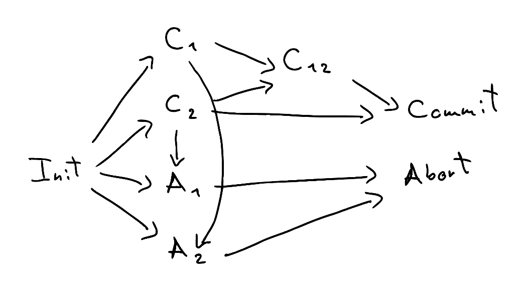
If we want to model the protocol at a higher level, we can decide to not keep track of the client state:
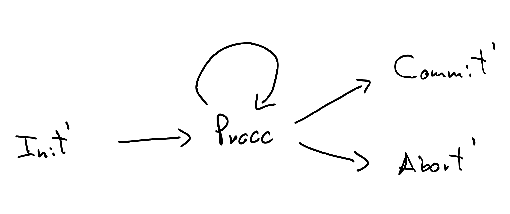
We then need a way to relate the two models: we can use similarity to that effect. We can see that \( Init \le Init' \), all the C and A states are simulated by Procc, \( Commit \le Commit' \), and \( Abort \le Abort' \). For example, the sequence \( [Init, C_1, A_2, Abort] \) is simulated by \( [Init', Procc, Procc, Abort'] \).
Working in the complete powerset lattice \( \mathcal{P}(Pr \times Pr) \), we can obtain similarity as the greatest fixpoint of a functional \( F : \mathcal{P}({Pr \times Pr}) \rightarrow \mathcal{P}({Pr \times Pr}) \) given by The intuition for \( F(R) \) is that it gives us all pairs \( (P, Q) \) where \( Q \) can simulate \( P \) for one step and after that one step we end up in a pair of states in \( R \). \[ F(R) = \{ (P, Q) | \forall P', P \rightarrow_\mu P' \implies \exists Q'. Q \rightarrow_\mu Q' \land (P', Q') \in R \} \]
Fact 1. \( F \) is monotone. This means that if \( S \subseteq R \) then \( F(S) \subseteq F(R) \).
Fact 2. \( R \) is a simulation iff \( R \) is a post-fixpoint of \( F \) (i.e. \( R \subseteq F(R) \) ).
Corollary 3. similarity is F's greatest fixpoint (follows by Knaster-Tarski).
Moreover, we can stratify similarity through a family of relations \( \{ \le_n \} \) capturing similarity up to \(n\) steps:
- \( \le_0 = Pr \times Pr \)
- \( \le_{n + 1} = F(\le_n) \)
To compute similarity, we'd like to know that \( P \le Q \) iff \( P \le_n Q \) for all n; i.e. $$ \le = \bigcap_{i \ge 0} \le_i $$ If so, we could compute \( \le_0, \le_1, \ldots, \le_n, \ldots \) Since \( F \) is monotone, then we can stop computing as soon as we reach a fixpoint \( \le_n = F(\le_{n}) = \le_{n + 1} \), In that case $$ \le = \bigcap_{i \ge 0} \le_i = \le_n $$ This is justified by the following lemma:
Lemma 4. For \( i \ge 0 \), if \( P \le_{i + 1} Q \), then \( P \le_i Q \).
Proof. Intuitively, this makes sense. If \( Q \) can simulate \( P \) for \( i + 1 \) steps, then surely it can also simulate it for \( i \) steps. Formally, we have to show that \( \le_{i + 1} \subseteq \le_i \). Note that $$ \le_1 \subseteq Pr \times \Pr = \le_0 $$ Since \( F \) is monotone we can (repeatedly) apply it on both sides to get $$ \begin{align} \le_2 = F(\le_1) \subseteq F(\le_0) = \le_1 \\ \le_3 = F(\le_2) \subseteq F(\le_1) = \le_2 \\ \ldots \end{align} $$ The proof follows by induction. \( \blacksquare \)
Corollary 5. If \( n \ge m \), then \( P \le_n Q \) implies \( P \le_m Q \).
The fixpoint algorithm can be implemented more or less verbatim (below in Scala, full source here):
// Compute the similarity relation on nodes of a
// labelled-transition system (LTS) via fixpoints.

object Trans {
  // LTS processes and actions
  type Procc = String
  type Act = Int

  // A labelled-transition system is a set of processes (nodes)
  // and transitions between them.
  case class LTS(
    procc: Set[Procc],
    trans: Map[Procc, List[(Act, Procc)]])

  // A relation is a set of pairs of processes.
  type Rel = Set[(Procc, Procc)]
}

import Trans._

class Simil(L1: LTS, L2: LTS) {
  // The _functional_ computes the pairs (p, q) where
  // q simulates p for one step and we end up in elements
  // in R.
  def funct(R : Rel): Rel = {
    for {
      s1 <- L1.procc
      s2 <- L2.procc
      if L1.trans.getOrElse(s1, List()).forall(
        { case (a1, p1) =>
          // s1 ->_a1 p1
          L2.trans.getOrElse(s2, List()).exists(
            { case (a2, p2) =>
              // s2 ->_a2 p2
              a2 == a1 && R.contains(p1, p2)  })
        })
    } yield (s1, s2)
  }

  // Compute the fixpoint of a function f from the sequence
  // [R, f(R), f(f(R)), ...]
  @tailrec
  private def fixpoint(R : Rel, f : Rel => Rel): Rel = {
    val next = f(R)
    if (next == R) R else fixpoint(next, f)
  }

  // Compute the similarity relation between processes in
  // two LTSs (i.e. which processes in the second LTS simulate
  // the ones in the first).
  val simil: Rel = {
    // Initially, consider all pairs of processes.
    var R0: Rel = for {
      p1 <- L1.procc
      p2 <- L2.procc
    } yield (p1, p2)
    // Now iterate until we reach a fixpoint.
    fixpoint(R0, funct)
  }
}
For the 2PC models above, we indeed get that \( Init \le Init' \) as expected. The full relation is { A1 ≤ Init', A1 ≤ Procc, A2 ≤ Init', A2 ≤ Procc Abort ≤ Abort', Abort ≤ Commit', Abort ≤ Init' Abort ≤ Procc, C1 ≤ Init', C1 ≤ Procc, C12 ≤ Init', C12 ≤ W, C2 ≤ Init', C2 ≤ Procc, Commit ≤ Abort', Commit ≤ Commit', Commit ≤ Init', Commit ≤ Procc, Init ≤ Init', Init ≤ Procc }
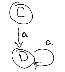
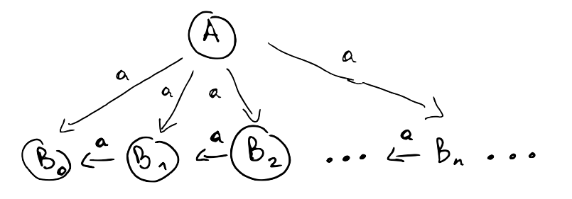
Unfortunately the method above doesn't always work. In the example below, \( A \) can take \( n \) a-steps for any \( n \), so \( C \le_n A \) and \( (C, A) \in \bigcap_{ i \ge 0} \le_i \). However, \( A \) cannot simulate \( C \) because \( C \) can take infinitely many steps whereas \( A \) needs to "commit" to one of the \( B_i \), and from then on it can only take a finite number of steps.
To see what the problem is, it helps to try to carry out the proof that \( \le = \bigcap_{i \ge 0} \le_i \) and see where it breaks. For this, we need to show that \( \le \subseteq \bigcap_{i \ge 0} \) and \( \bigcap_{i \ge 0} \subseteq \le \). The first goal goes through without problems. Notice that $$ \begin{align} \le & \subseteq Pr \times Pr &= \le_0 \\ \le = F(\le) & \subseteq F(\le_0) &= \le_1 \\ \le = F(\le) & \subseteq F(\le_1) &= \le_2 \\ \ldots & & \end{align} $$ Using the fact that \( \le \) is a fixpoint and \( F \) is monotone we can proceed by induction to show that \( \le \subseteq \le_n \) for all \( n \), and the result follows.
It's the second goal that gives us trouble. We need to show that \( \bigcap_{i \ge 0} \le_i \subseteq \le \). Since similarity is the largest simulation, it's enough to show that \( \bigcap_{i \ge 0} \le_i \) is a simulation. That is, given that \( (P, Q) \in \bigcap_{i \ge 0} \le_i \) and assuming that \( P \rightarrow_\mu P' \), we have to show that there exists a Q' such that \( Q \rightarrow_\mu Q\ \) and \( (Q, Q') \in \bigcap_{i \ge 0} \le_i \). Because \( (P, Q) \in \bigcap_{i \ge 0} \le_i \) we know that for each \(i\) we can find a \( Q'_i \) such that \( Q \rightarrow_\mu Q'_i \) and \( (P', Q'_i ) \in \le_i \). That is, we know $$ \forall i. \exists Q'. Q \rightarrow_\mu Q' \land (P', Q') \in \le_i $$ But we need $$ \exists Q'. \forall i. Q \rightarrow_\mu Q' \land (P', Q') \in \le_i $$ Of course, we know we can't simply swap the quantifiers, which is consistent with the counterexample we saw above. In the counterexample, process \( A \) had infinitely-many outgoing transitions, so one (not very intuitive) question to ask is whether restricting the LTS to being finitely branching solves the problem (it does).
Definition 6. An LTS is finitely branching if for every process \( P \) the set \( \{ (\mu, Q) | P \rightarrow_\mu Q \in \rightarrow \} \) is finite.
We now finally get to the meat of the matter: if the LTS is finitely branching, then we can exchange the quantifiers.
Lemma 7. If the underlying LTS is finitely branching, then $$ \forall i. \exists Q'. Q \rightarrow_\mu Q' \land (P', Q') \in \le_i $$ implies $$ \exists Q'. \forall i. Q \rightarrow_\mu Q' \land (P', Q') \in \le_i $$ Proof. Let \( M = \{ Q\ | Q \rightarrow_\mu Q' \in \rightarrow \} \). Since the LTS is finitely branching, then \( M \) is finite. From the assumption, we can construct a function \( f(i) = Q_i \) that assigns to every index \( i \) an element \( Q_i \in M \) such that \( Q \rightarrow_\mu Q_i \land (P', Q_i) \in \le_i \). Now define the fiber \( f^{-1}(e) \) of an element \( e \) to be the inverse image of the singleton set containing \( e \): $$ f^{-1}(Q') = \{ i | f(i) = Q' \} $$ Notice that the set of natural numbers can be partitioned as the union of the fibers of elements of \( M \): $$ \mathbb{N} = \bigcup_{Q' \in M} f^{-1}(Q') $$ Now look at the cardinalities on each side of the equation above. \( \mathbb{N} \) is infinite, and there are finitely many \( Q' \in M \). This means that at least one of the elements has an infinite fiber. Let \( Q' \) be one such element. Now consider an arbitrary index \( i \). Since \( f^{-1}(Q') \) is infinite, there exists a \( j > i \) such that \( j \in f^{-1}(Q') \), meaning that \( f(j) = Q' \). In turn, this means that $$ Q \rightarrow_\mu Q' \land (P', Q') \in \le_i $$ Since \( i \) was arbitrarily chosen, we get $$ \forall i, Q \rightarrow_\mu Q' \land (P', Q') \in \le_i $$ which is allows us to instantiate the existential in our goal. \( \blacksquare \)
The abstract view of Lemma 7 above is given in Theorem 1 (Regular Quantification) of Amin's blog post:
Let A be a regular ordinal, [...] and B be a set with strictly smaller cardinality [...]. The following holds for any \( P \) that is downwards closed with respect to the relation on A: $$ (\forall x \in A. \exists y \in B. P(x, y) ) \implies \exists y \in B. \forall x \in A. P(x, y) $$
Contrast with a version of Lemma 7 massaged to highlight the parallels $$ ( \forall i \in \mathbb{N}. \exists Q' \in succ(Q, \mu). \mathcal{S}(i, Q') ) \implies \exists Q' \in succ(Q, \mu). \forall i \in \mathbb{N}. \mathcal{S}(i, Q') $$ where $$ \begin{align} succ(Q, \mu) &= \{ Q' | Q \rightarrow_\mu Q' \} \\ \mathcal{S}(i, Q') &= (P', Q') \in \le_i \end{align} $$
In order to use Theorem 1, we need
- \( \mathbb{N} \) must be a regular ordinal. For our purposes, this means the following: suppose we have an unbounded subset \( S \) of \( \mathbb{N} \) (i.e. for any natural number \( n \) no matter how large, we can always find an element \( e \in S \) such that \( e > n \)). Then we need to show there exists an injective function \( f : \mathbb{N} \rightarrow S \). We can recursively construct one such function. We will set \( f(0) \) to an arbitrary element of \( S \). For the recursive case, we are given \( f(n - 1) \) and have to define \( f(n) \). Since \( S \) is unbounded, there's an element \( e \in S \) such that \( e > f(n - 1) \). We set \( f(n) = e \). It's easy to see that if \( n < m \) then \( f(n) < f(m) \); this means \( f \) is injective as needed. \( \blacksquare \)
- \( succ(Q, \mu) \) must have strictly smaller cardinality than \( \mathbb{N} \). This is easy, because since the LTS is finitely branching \( succ(Q, \mu) \) must be finite, and \( \mathbb{N} \) is infinite. \( \blacksquare \)
- \( \mathcal{S}(i, Q') \) is downwards-closed. Here we need to show that if \( n \ge m \) then $$ P' \le_n Q' \implies P' \le_m Q' $$ This is precisely the previously shown Corollary 5. \( \blacksquare \)
References
- Sangiorgi, Davide. Introduction to Bisimulation and Coinduction. Cambridge University Press, 2011.
- Timany, Amin. Commuting Quantifiers. https://tildeweb.au.dk/au571806/blog/commuting_quantifiers/.
- Lamport, Leslie. Specifying systems. Vol. 388. Boston: Addison-Wesley, 2002. https://lamport.azurewebsites.net/tla/book.html